
The concept of Electromagnetic Fields in a PCB
Categories: Electromagnetism, EMC/EMI Design · Tags: EMI, EMC, PCB DESIGN
Note: The article you are about to read is directly extracted from one of the lessons in the comprehensive EMC/EMI Design Course. Visit the course page to find out how to enroll.
Introduction: The Foundation of Low-EMI PCB Design
One of the most important concepts in designing printed circuit boards (PCBs) for low electromagnetic interference (EMI) is understanding electromagnetic fields, specifically, how to contain and control them. EMI is fundamentally about field containment: controlling where fields need to be strong and where they need to be weakened. When we discuss fields, we're referring to both electric and magnetic fields. Therefore, if our goal is to design PCBs with low EMI, we must understand how these fields behave and how to control them. By mastering this understanding, we can achieve high-performing circuits that pass electromagnetic compatibility (EMC) tests, an essential requirement before any product can be sold in the marketplace.
Visualizing Electromagnetic Fields
One of the most effective approaches to understanding electromagnetic (EM) fields is to visualize them. While these phenomena can be complex, simplified visual representations help us grasp the fundamentals that are essential when designing or debugging products for low EMI.
Single Conductor Field Behavior
The first visualization we need to understand shows how fields surround a single conductor.
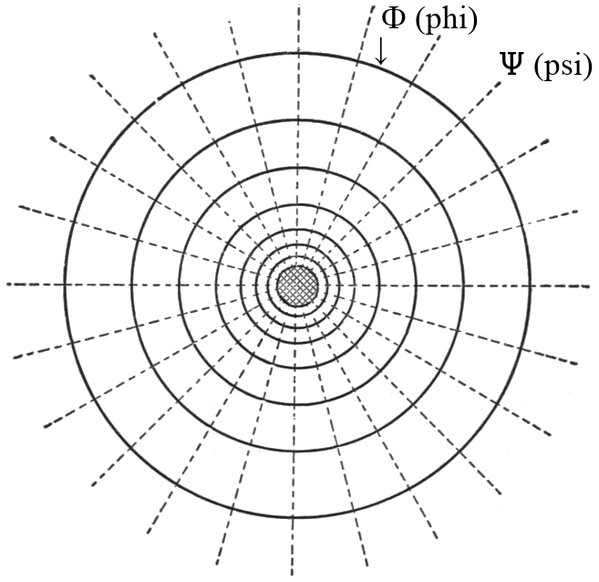
[ Φ magnetic flux; Ψ dielectric flux; from Steinmetz (1911, p.10) ]
In this scenario, the circle at the center represents a conductor viewed in cross-section. Surrounding this conductor are the magnetic and electric fields, which together form the electromagnetic field.
The magnetic field is quantified by the number of lines of magnetic force, denoted by the symbol Φ (PHI). These magnetic field lines encircle the conductor, forming closed loops that represent the magnetic flux generated by the current flowing through the conductor.
The electric field is represented by dashed lines in the diagram. These lines originate from the conductor and are measured by the number of lines of electric force, denoted by the symbol Ψ (PSI). In the case of a single conductor, the electric field lines radiate outward as straight lines from the conductor.
Two-Conductor System: The Return Path Effect
However, when a return conductor is introduced, the behavior of the fields changes dramatically, as illustrated in Figure 2.
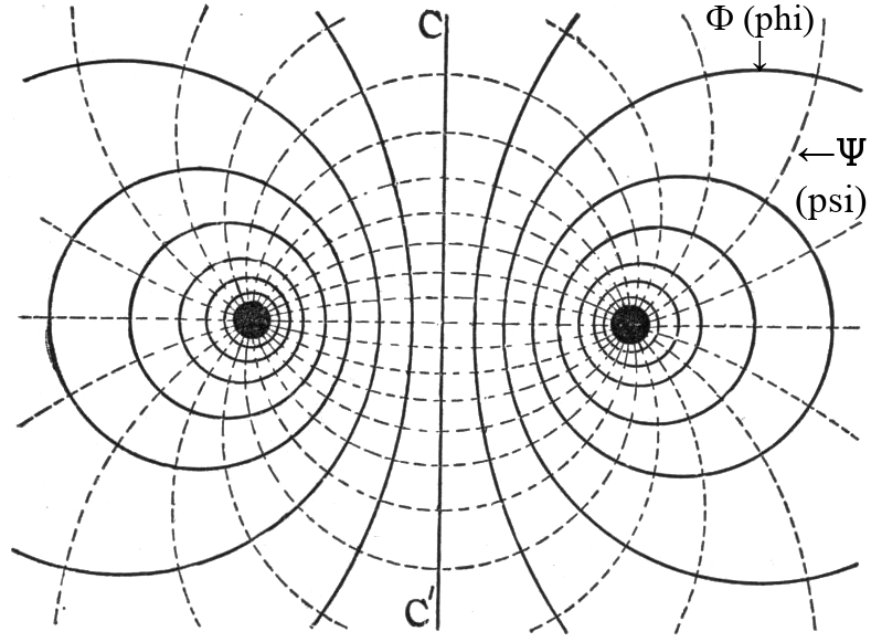
[ Φ magnetic flux; Ψ electric flux; from Steinmetz (1911, p.11) ]
In this two-conductor scenario:
-
Magnetic field lines become concentrated between the two conductors, forming stronger, more focused loops in the space between them. Outside of this space, the magnetic field lines spread out more broadly.
-
Electric field lines change their behavior significantly. Instead of radiating outward from a single conductor, the electric field lines now start from one conductor and terminate at the other.
Key Field Characteristics
The key takeaway from these visualizations is fundamental: magnetic field lines always form closed loops, while electric field lines terminate at conductors.
This distinction leads us to describe:
-
The magnetic field as a "magnetic circuit," where field lines loop continuously
-
The electric field as an "electric circuit," where field lines originate and terminate at specific points
Field Polarity and Interaction
Opposite Polarities: Field Termination
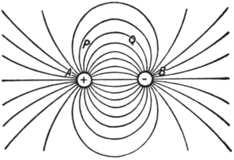
When conductors have opposite polarities, electric field lines originate from one polarity and terminate on the opposite polarity. This demonstrates how fields interact between positive and negative conductors, with lines of force creating a direct path between them.
Like Polarities: Field Repulsion
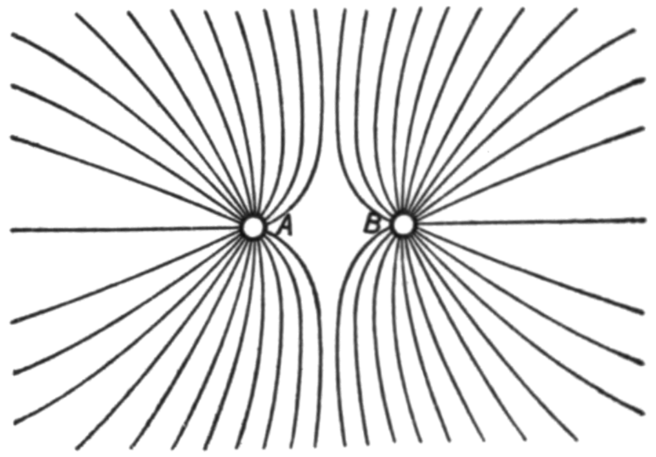
Conversely, when two conductors have the same polarity, the fields repel each other. The electric field lines push away from each other, illustrating how like charges repel and how this affects the distribution of the electric field.
Application to PCB Design
Basic PCB Field Behavior
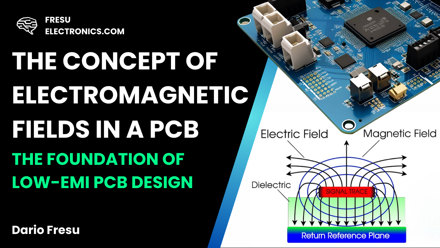
These fundamental principles apply directly to printed circuit board design, as shown in Figure 5.
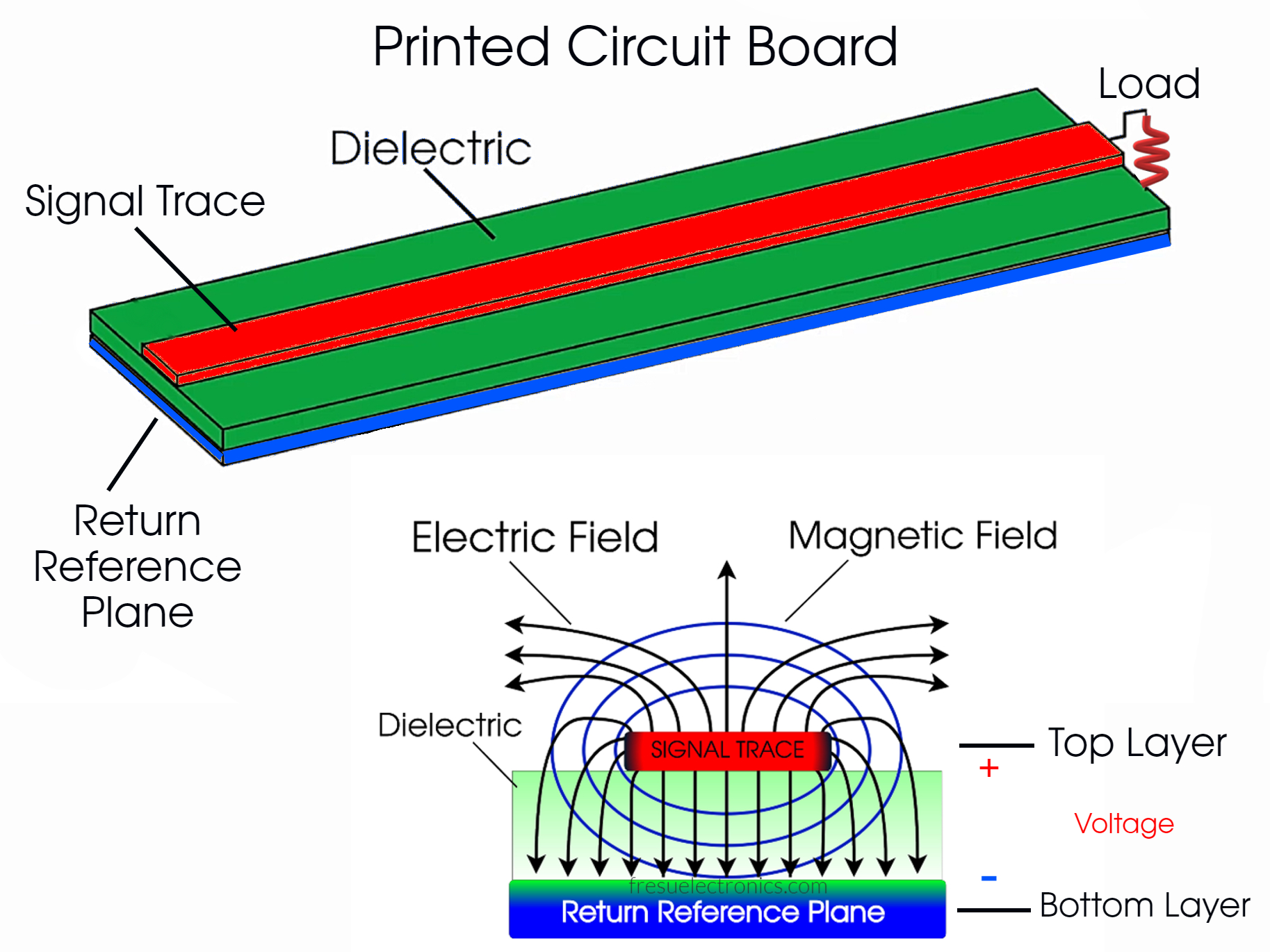
This representation shows a PCB formed by a two-layer stackup consisting of:
-
A signal layer (shown in red) containing the signal traces
-
A return reference plane (depicted in blue)
The term "stackup" refers to the specific arrangement of PCB layers, including the conductive copper layers where signal traces and reference planes are located, as well as the insulating layers and prepreg or core materials that separate and support these conductive layers.
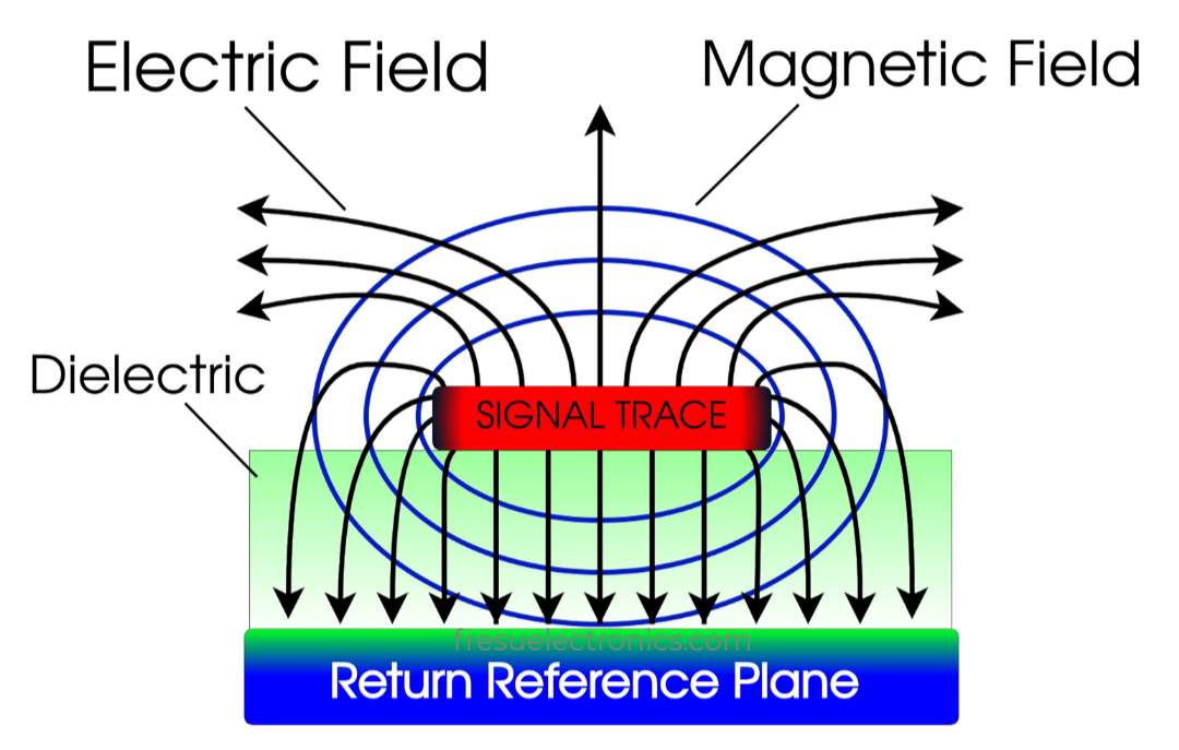
When we observe the fields in this PCB configuration, the behavior is similar to the two-conductor scenario shown in Figure 2. However, in this instance, the two conductors are oriented at a 90-degree angle.
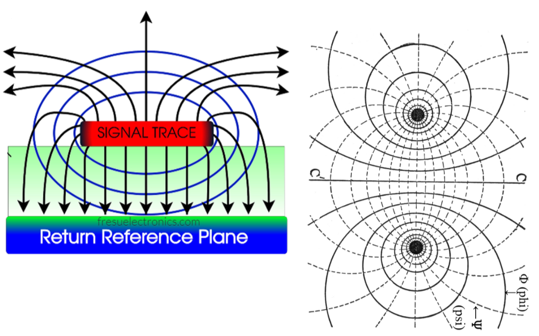
This comparison lays the foundation for understanding how to design PCBs with low EMI. Our objective is to design the PCB to contain and redirect the fields exactly where we want them by carefully shaping the geometries of the circuit board.
The Critical Role of Return Reference Planes
Field Containment Mechanism
In practical terms, the fields of the signal trace in a PCB are significantly influenced by the return reference plane. The fields not only terminate at the surface of the return plane but also tend to bend towards it from the opposite side. This bending effect helps contain the fields and prevents them from spreading outward as they would in the absence of the return plane. The return reference plane acts as a boundary that contains the fields, preventing them from dispersing freely into the surrounding space. Without this plane, the fields would continue spreading outward from the signal trace, as illustrated in Figure 1.
The Consequences of Missing Return Planes
Understanding how fields are contained by the return reference plane is essential for PCB design. The choice of stackup—how the layers of the board are arranged—must be based on this principle.
The key takeaway: Removing the return reference plane allows the fields to expand uncontrollably. This is a major reason why PCBs often fail EMC tests and generate EMI issues. Signal traces without an adjacent return reference plane lack the necessary containment for the fields, leading to excessive radiation.
When we measure fields during EMC testing, we often find that levels exceed requirements because, without a return reference plane, the PCB effectively becomes a radiator, emitting unwanted electromagnetic energy.
Real-World Implications
In practical scenarios, particularly with common electronic consumer products, if a PCB lacks a return reference plane adjacent to the signal traces, the earth ground will act as the return path. This causes the fields to continue expanding until they eventually reach the earth ground or other nearby conductive structures. This expansion can lead to the formation of common-mode currents, which are highly effective at radiating electromagnetic energy. These currents can easily cause a product to fail EMC tests if the radiated fields exceed acceptable limits.
The Fundamental Design Rule
To mitigate EMI issues, the first and most important rule of thumb in PCB design is:
For each signal layer, there must be a return reference plane adjacent to it. This return plane should be free of discontinuities, such as large holes, gaps, cuts, or any other malformations that could compromise its effectiveness.
The return reference plane should be as integral and as close as possible to the signal trace. This approach is key to successfully passing EMC tests on the first attempt. Proper design with an adjacent, continuous return reference plane ensures that fields are effectively contained, reducing the chances of EMI issues.
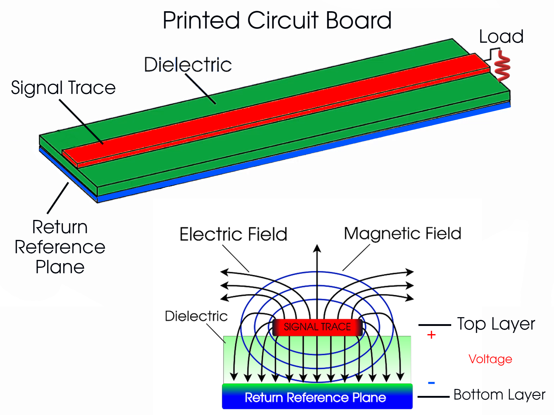
This final image highlights a crucial concept to remember when designing printed circuit boards. It visually emphasizes the significance of field containment through an appropriate layer stackup, which is essential for effective low-EMI PCB design. Additionally, a key point to be explored further in other lessons and articles is that energy is carried by the fields, not within the conductor. Instead, it resides in the medium between the conductors, where permittivity and permeability control the energy transfer. At Fresu Electronics, we are dedicated to helping engineers grasp and implement best design practices from the outset. If you're interested in enhancing your skills, we invite you to explore our courses and EMI control guides.